|
|
|


|
10-3 kg/(m·s)
|
||
|
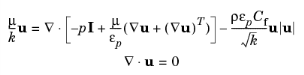
εp
|
||

|
1
|
|
2
|
|
3
|
|
4
|
Click Study.
|
|
5
|
|
6
|
Click Done.
|
|
1
|
|
2
|
|
3
|
|
4
|
|
5
|
|
1
|
|
2
|
|
3
|
|
4
|
|
5
|
|
6
|
|
7
|
|
1
|
|
2
|
|
1
|
In the Model Builder window, under Component 1 (comp1) right-click Materials and choose Blank Material.
|
|
2
|
|
1
|
|
2
|
|
1
|
|
2
|
|
3
|
|
1
|
|
3
|
|
4
|
|
5
|
Locate the Porous Matrix Properties section. From the Porous material list, choose Porous Matrix (mat2).
|
|
1
|
|
2
|
|
1
|
|
2
|
|
1
|
|
2
|
|
3
|
|
1
|
|
3
|
|
4
|
|
1
|
|
1
|
In the Model Builder window, under Component 1 (comp1) right-click Mesh 1 and choose Free Triangular.
|
|
2
|
|
3
|
Click the Custom button.
|
|
4
|
|
5
|
|
1
|
|
2
|
|
3
|
Click Add.
|
|
5
|
|
1
|
|
2
|
|
3
|
|
1
|
|
2
|
|
3
|
|
4
|
|
1
|
|
2
|
|
3
|
|
4
|
|
1
|
|
2
|
|
1
|
|
2
|
|
3
|
|
4
|
|
5
|
Click to expand the Coloring and style section. Locate the Coloring and Style section. From the Marker list, choose Cycle.
|
|
6
|
|
7
|
|
9
|