PDF

Biot Poroelasticity
Introduction
Poroelastic models describe the linked interaction between fluids and deformation in porous media. The fluids in a reservoir absorb stress, which registers as fluid pressure or equally hydraulic head. For example, if pumping significantly reduces pore fluid pressures, sediments could shift due to the increased load. Because the reduction in the pore space brings about more fluid movement, the reservoir could compact further. It follows that lateral stretching must compensate for the vertical compaction.
Model Definition
This example analyzes fluid and solid behavior within three sedimentary layers overlying an impermeable bedrock in a basin. The bedrock is faulted, which creates a step near a mountain front. The sediment stack totals 420 m at the centerline of the basin (x = 0 m) and thins to 120 m above the step (x > 4000 m). The top two layers are each 20 m thick.
Figure 1: Model geometry showing boundary segments (from Leake and Hsieh, Ref. 1).
Pumping from the lower aquifer reduces hydraulic head down the centerline of the basin by 6 m per year. The head drop moves fluid away from the step. The middle layer is relatively impermeable. The pumping does not diminish the supply of fluids in the unpumped reservoir above it. The flow field is initially at steady state. The period of interest is 10 years.
Governing Equations
This example uses the Poroelasticity multiphysics node, which includes the time rate of change in strain from the Solid Mechanics interface in the Darcy’s Law interface and adds the fluid pressure gradient as stress contribution in the Solid Mechanics interface. The following sections describe the built-in equations when using the Poroelastic Material feature as well as the initial and boundary conditions.
Fluid Flow
Use the Darcy’s Law interface to estimate the flow field in the poroelastic model with the pressure head formulation
(1)
where ρf is the fluid density, H is the pressure head (m), K is the hydraulic conductivity (m/s), εvol is the volumetric strain of the porous matrix, and αB is the Biot-Willis coefficient; in this model the Biot-Willis coefficient equals 1, which is a common value for “soft soils.” You can interpret the term on the right-hand side as the time rate of expansion of the porous matrix. The volume fraction available for liquid increases and thereby gives rise to liquid sink, which is why the sign is reversed in the source term. Leake and Hsieh (Ref. 1) defined Sα using coefficients from the solids equation, the Young’s modulus, E, and Poisson’s ratio, ν. Debate over poroelastic storage coefficients is heated (Ref. 2), and the subscript α here denotes that conventional storage terms might need redefinition for poroelasticity models.
The main differences between the Terzaghi compaction model and this poroelastic analysis lie in material coefficients and sources; the boundary conditions are identical: H is the offset in hydraulic head since an initial steady-state distribution of H0. This subtle twist simplifies describing the boundary conditions: the value at the outlet boundary becomes the decline in hydraulic head with time, and at the upper aquifer, the hydraulic head is fixed at H0. All other boundaries have no-flow conditions. The boundary and initial conditions for the Darcy’s law analysis are
where n is the normal to the boundary. The letters A through E come from Leake and Hsieh (Ref. 1), each letter denoting a specific boundary (see Figure 1).
Porous matrix Deformation
The governing equation for the poroelastic material model is
(2)
here, σ is the stress tensor, ρ is the total density, and g is acceleration of gravity. The poroelastic material model uses Equation 2 to describe changes in the stress tensor σ and porous matrix displacement u due to boundary conditions and changes in pore pressure. This focus on changes in displacement is standard poroelasticity and greatly simplifies specifying loads, boundaries, and initial conditions. Equation 2 defines a state of static equilibrium because the changes in the solid equilibrate quickly, unlike vibrations or waves, that is, there are no time-dependent terms. Still the time rate of change in strain ∂εvol/∂t appears as a coupling term in Darcy’s Law because the solids equation becomes quasi-static when solved simultaneously with a time-dependent flow model.
The governing equation for the bedrock step problem describes the deformation state of plane strain, which is the norm for 2D poroelasticity problems (Ref. 1 and Ref. 2), so the strain normal to the xy-plane equals zero. COMSOL Multiphysics solves Equation 2 using the Solid Mechanics interface.
For an isotropic porous material under plane strain conditions, this simplifies to
(3)
where E is Young’s modulus (Pa) and ν is Poisson’s ratio of the drained porous matrix. The term αBp (Pa) amounts to the fluid pressure contribution and is often described as the fluid-to-structure coupling expression. This contribution is added by the Poroelasticity multiphysics node.
With small deformations for plane strain analyses, the normal strains εxx, εyy, εzz and shear strains εxy, εyz, εxz relate to the displacements u and v as
(4)
Inserting the relationships from Equation 3 and Equation 4 into Equation 2 gives the equation that COMSOL Multiphysics solves.
The boundary conditions on the porous matrix are a series of constraints on the displacement that allow for horizontal movement at the surface and throughout the basin. The base of the sediments is fixed, which means you constrain horizontal and vertical displacement to zero. The upper surface is free to vary in the horizontal and the vertical directions. The boundary on left of Figure 1 is a roller condition, so the sediments are free to move in the vertical direction, but there is no horizontal displacement. These conditions result in the following boundary expressions
where, once again, the letters A through E come from Leake and Hsieh, and denote the boundaries in Figure 1.
Model Data
The coefficients and parameters for the poroelasticity model are as follows:
ρf
ρd
1·10-6 m-1
Sα
1·10-5 m-1
αB
H0
H(t)
8·108 Pa
8·107 Pa
ν
Results and Discussion
Figure 2, Figure 3, and Figure 4 are Year 2, Year 5, and Year 10 snapshots, respectively, from the COMSOL Multiphysics solution to the problem (Ref. 1) of linked fluid flow and solid deformation near a bedrock step in a sedimentary basin. The shading and arrows, respectively, represent the change in hydraulic head and velocities brought about by pumping from the basin interior at x = 0 m. The fluid moves from the surface toward the well screens in the lower aquifer, with an abrupt change in direction and velocity near the bedrock step. In this way, the flow solution here is similar to the results in Terzaghi compaction model.
The results for the solids displacement tell another story. In Figure 2, Figure 3, and Figure 4, contours and deformed shapes illustrate the total displacement. The plot sequence illustrates the evolution of lateral deformations that compensate for the changing surface elevation above the bedrock step.
Figure 2: Solution for a poroelasticity analysis of the bedrock step problem of Leake and Hsieh (Ref. 1): Hydraulic head (surface plot), displacement (contours and deformations) at Year 2. The vertical axis is expanded for clarity.
Figure 3: Hydraulic head (surface plot), displacement (contours and deformations) at Year 5. The vertical axis and deformation are exaggerated for clarity.
Figure 4: Hydraulic head (surface plot), displacement (contours and deformations) at Year 10. The vertical axis and deformation are exaggerated for clarity.
Figure 5, represents the coupling terms that link the fluid and structure equations. The shading gives the structure-to-fluid link, which is the negative of the time rate of change in strain (see Equation 1).
Figure 5: The solid-to-fluid coupling term evaluated at Year 10 with the poroelastic analysis. The squeeze of porous matrix results in an apparent mass source term.
The Terzaghi and Biot solutions differ most when it comes to predicting the horizontal strain at the edge of the bedrock step. The Biot poroelasticity analysis predicts horizontal strain; the Terzaghi compaction analysis does not. The horizontal strains at the ground surface from the Biot poroelasticity approach appear in Figure 6. It depicts negative strain or compaction immediately on the basin side of the step; the positive strains correspond to tension or lengthening on the mountain side.
Figure 6: COMSOL Multiphysics estimates of horizontal strain from poroelastic analysis for the bedrock step problem of Leake and Hsieh: Year 2 (blue, solid line), Year 5 (green, dotted line), and Year 10 (red, dashed line).
Failure criteria or expressions defining a critical threshold for stress, strain, or displacements facilitate evaluating whether the strain differential at the bedrock steps is big enough to produce fissures. Figure 7 plots von Mises stresses (surface plot), fluid velocities (streamlines), and total displacement (deformation). The von Mises stresses are postprocessing variables defined by COMSOL Multiphysics in all structural-deformation analyses. The von Mises stresses are variables in many failure expressions and you can also use them as yield functions in the elasto-plastic materials dialog boxes.
Figure 7: COMSOL Multiphysics estimates of von Mises stresses (surface plot), fluid velocities (streamlines), and displacement (deformation) at Year 10. These results correspond to the poroelastic analysis from Leake and Hsieh (Ref. 1). The vertical axis and deformation are exaggerated for clarity.
References
1. S.A. Leake and P.A. Hsieh, Simulation of Deformation of Sediments from Decline of Ground-Water Levels in an Aquifer Underlain by a Bedrock Step, U.S. Geological Survey Open File Report 97-47, 1997.
2. H.F. Wang, Theory of Linear Poroelasticity with Application to Geomechanics and Hydrogeology, Princeton Univ. Press, 2000.
Application Library path: Subsurface_Flow_Module/Flow_and_Solid_Deformation/biot_poroelasticity
Modeling Instructions
Root
1
From the File menu, choose Open.
2
Results
Contour 1
Add a Solid Mechanics interface and a Poroelasticity multiphysics node.
Add Physics
1
On the Home toolbar, click Add Physics to open the Add Physics window.
2
Go to the Add Physics window.
3
In the tree, select Structural Mechanics>Solid Mechanics (solid).
4
Click Add to Component in the window toolbar.
Solid Mechanics (solid)
1
On the Home toolbar, click Add Physics to close the Add Physics window.
2
On the Home toolbar, click Add Multiphysics.
Add Multiphysics
1
Go to the Add Multiphysics window.
2
In the tree, select Structural Mechanics>Poroelasticity.
3
Click Add to Component in the window toolbar.
Multiphysics
1
On the Home toolbar, click Add Multiphysics.
The insertion of the multiphysics node automatically inserts a poroelastic storage material model in Darcy’s Law and sets the Discretization to ’linear’.
Darcy’s Law (dl)
On the Physics toolbar, click Solid Mechanics (solid) and choose Darcy’s Law (dl).
Poroelastic Storage 1
1
In the Model Builder window, expand the Darcy’s Law (dl) node, then click Poroelastic Storage 1.
2
In the Settings window for Poroelastic Storage, locate the Fluid Properties section.
3
From the Fluid material list, choose Fluid (mat1).
4
Locate the Matrix Properties section. From the Permeability model list, choose Hydraulic conductivity.
5
In the K text field, type K_s.
Solid Mechanics (solid)
On the Physics toolbar, click Darcy’s Law (dl) and choose Solid Mechanics (solid).
Gravity 1
1
On the Physics toolbar, click Domains and choose Gravity.
2
In the Settings window for Gravity, locate the Domain Selection section.
3
From the Selection list, choose All domains.
Fixed Constraint 1
1
On the Physics toolbar, click Boundaries and choose Fixed Constraint.
2
Roller 1
1
On the Physics toolbar, click Boundaries and choose Roller.
2
Multiphysics
1
In the Model Builder window, under Component 1 (comp1)>Multiphysics click Poroelasticity 1 (poro1).
2
In the Settings window for Poroelasticity, locate the Poroelastic Coupling Properties section.
3
From the αB list, choose User defined. In the associated text field, type 1.
Fill the required fields in the material properties tables.
Materials
Fluid (mat1)
1
In the Model Builder window, under Component 1 (comp1)>Materials click Fluid (mat1).
2
In the Settings window for Material, locate the Material Contents section.
3
Porous 1 (mat2)
1
In the Model Builder window, under Component 1 (comp1)>Materials click Porous 1 (mat2).
2
In the Settings window for Material, locate the Material Contents section.
3
Porous 2 (mat3)
1
In the Model Builder window, under Component 1 (comp1)>Materials click Porous 2 (mat3).
2
In the Settings window for Material, locate the Material Contents section.
3
Create a variable to calculate the solid-to-fluid coupling term.
Definitions
Variables 3
1
In the Model Builder window, expand the Component 1 (comp1)>Definitions node, then click Variables 3.
2
In the Settings window for Variables, locate the Variables section.
3
Study 1
Disable the newly created nodes in the existing study.
Step 1: Time Dependent
1
In the Model Builder window, expand the Study 1 node, then click Step 1: Time Dependent.
2
In the Settings window for Time Dependent, locate the Physics and Variables Selection section.
3
In the Physics interface table, clear the Solve for check box for Solid Mechanics (solid).
4
In the Multiphysics table, clear the Solve for check box for Poroelasticity 1 (poro1).
5
Select the Modify physics tree and variables for study step check box.
6
In the Physics and variables selection tree, select Component 1 (comp1)>Darcy’s Law (dl)>Poroelastic Storage 1.
7
Click Disable.
Add Study
1
On the Home toolbar, click Add Study to open the Add Study window.
2
Go to the Add Study window.
3
Find the Studies subsection. In the Select Study tree, select Preset Studies>Time Dependent.
4
Click Add Study in the window toolbar.
Study 2
Step 1: Time Dependent
1
On the Home toolbar, click Add Study to close the Add Study window.
2
In the Model Builder window, under Study 2 click Step 1: Time Dependent.
3
In the Settings window for Time Dependent, locate the Study Settings section.
4
From the Time unit list, choose a.
5
Click Range.
6
In the Range dialog box, type 1 in the Step text field.
7
In the Stop text field, type 10.
8
Click Replace.
9
On the Home toolbar, click Compute.
Results
Pressure (dl)
Follow the steps below to reproduce the plots shown in Figure 2 through Figure 4.
1
In the Model Builder window, under Results click Pressure (dl).
2
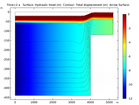
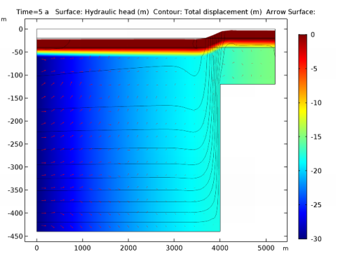
In the Settings window for 2D Plot Group, type Hydraulic Head, Poroelasticity in the Label text field.
Surface
1
In the Model Builder window, expand the Results>Hydraulic Head, Poroelasticity node, then click Surface.
2
In the Settings window for Surface, click Replace Expression in the upper-right corner of the Expression section. From the menu, choose Model>Component 1>Darcy’s Law>dl.H - Hydraulic head.
Contour 1
1
In the Model Builder window, under Results right-click Hydraulic Head, Poroelasticity and choose Contour.
2
In the Settings window for Contour, click Replace Expression in the upper-right corner of the Expression section. From the menu, choose Model>Component 1>Solid Mechanics>Displacement>solid.disp - Total displacement.
3
Locate the Levels section. From the Entry method list, choose Levels.
4
In the Levels text field, type range(0,0.2,2.3).
5
Locate the Coloring and Style section. From the Coloring list, choose Uniform.
6
From the Color list, choose Black.
7
Clear the Color legend check box.
8
Click to expand the Quality section. From the Resolution list, choose Extra fine.
Arrow Surface 1
1
Right-click Hydraulic Head, Poroelasticity and choose Arrow Surface.
2
In the Settings window for Arrow Surface, locate the Expression section.
3
In the X component text field, type d(dl.H,X).
4
In the Y component text field, type d(dl.H,Y).
5
Locate the Arrow Positioning section. Find the X grid points subsection. In the Points text field, type 25.
Deformation 1
1
In the Model Builder window, under Results>Hydraulic Head, Poroelasticity right-click Surface and choose Deformation.
2
In the Settings window for Deformation, locate the Scale section.
3
Select the Scale factor check box.
4
5
Right-click Results>Hydraulic Head, Poroelasticity>Surface>Deformation 1 and choose Copy.
Arrow Surface 1
1
In the Model Builder window, under Results>Hydraulic Head, Poroelasticity right-click Contour 1 and choose Paste Deformation.
2
In the Settings window for Arrow Surface, locate the Coloring and Style section.
3
Select the Scale factor check box.
4
On the Hydraulic Head, Poroelasticity toolbar, click Plot.
5
Hydraulic Head, Poroelasticity
1
Right-click Results>Hydraulic Head, Poroelasticity>Arrow Surface 1 and choose Paste Deformation.
2
In the Settings window for 2D Plot Group, locate the Data section.
3
From the Time (a) list, choose 2.
4
On the Hydraulic Head, Poroelasticity toolbar, click Plot.
5
Click the Zoom Extents button on the Graphics toolbar.
Compare the resulting plot with that in Figure 2.
6
From the Time (a) list, choose 5.
7
On the Hydraulic Head, Poroelasticity toolbar, click Plot.
The plot in the Graphics window should now look like that in Figure 3.
8
From the Time (a) list, choose 10.
9
On the Hydraulic Head, Poroelasticity toolbar, click Plot.
Compare with Figure 4.
Next, modify the second default plot to reproduce Figure 7.
Stress (solid)
1
In the Model Builder window, under Results click Stress (solid).
2
In the Settings window for 2D Plot Group, type Von Mises Stress in the Label text field.
Von Mises Stress
In the Model Builder window, expand the Results>Von Mises Stress node.
Deformation
1
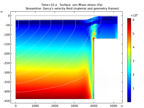
In the Model Builder window, expand the Results>Von Mises Stress>Surface 1 node, then click Deformation.
2
In the Settings window for Deformation, locate the Scale section.
3
Select the Scale factor check box.
4
Streamline 1
1
In the Model Builder window, under Results right-click Von Mises Stress and choose Streamline.
2
In the Settings window for Streamline, locate the Streamline Positioning section.
3
From the Positioning list, choose Start point controlled.
4
From the Entry method list, choose Coordinates.
5
In the X text field, type 0.
6
In the Y text field, type range(-450,50,-50).
7
Locate the Coloring and Style section. From the Color list, choose White.
8
Click to expand the Quality section. From the Smoothing list, choose Everywhere.
Deformation
In the Model Builder window, under Results>Von Mises Stress>Surface 1 right-click Deformation and choose Copy.
Deformation 1
In the Model Builder window, under Results>Von Mises Stress right-click Streamline 1 and choose Paste Deformation.
Next, reproduce the plot in Figure 5 showing the solid-to-fluid coupling term.
2D Plot Group 5
1
On the Home toolbar, click Add Plot Group and choose 2D Plot Group.
2
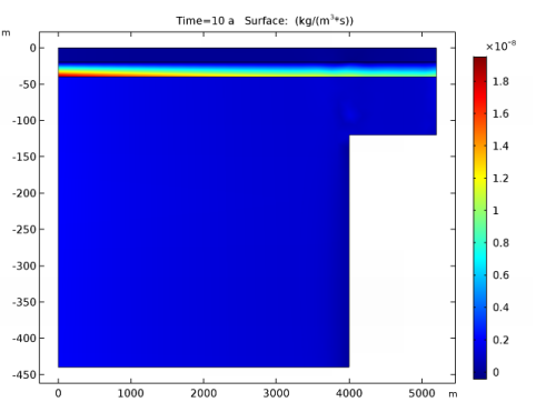
In the Settings window for 2D Plot Group, type Solid-to-Fluid Coupling Term in the Label text field.
3
Locate the Data section. From the Data set list, choose Study 2/Solution 2 (sol2).
Surface 1
1
Right-click Solid-to-Fluid Coupling Term and choose Surface.
2
In the Settings window for Surface, click Replace Expression in the upper-right corner of the Expression section. From the menu, choose Model>Component 1>Definitions>Variables>Q_biot.
3
On the Solid-to-Fluid Coupling Term toolbar, click Plot.
To set up the plot in Figure 6 proceed as follows:
Cut Line 2D 1
1
On the Results toolbar, click Cut Line 2D.
2
In the Settings window for Cut Line 2D, locate the Data section.
3
From the Data set list, choose Study 2/Solution 2 (sol2).
4
Locate the Line Data section. In row Point 1, set X to 1000.
5
In row Point 2, set X to 5000.
1D Plot Group 6
1
On the Results toolbar, click 1D Plot Group.
2
In the Settings window for 1D Plot Group, type Horizontal Strain in the Label text field.
3
Locate the Data section. From the Data set list, choose Cut Line 2D 1.
4
From the Time selection list, choose From list.
5
In the Times (a) list, choose 2, 5, and 10.
Line Graph 1
1
Right-click Horizontal Strain and choose Line Graph.
2
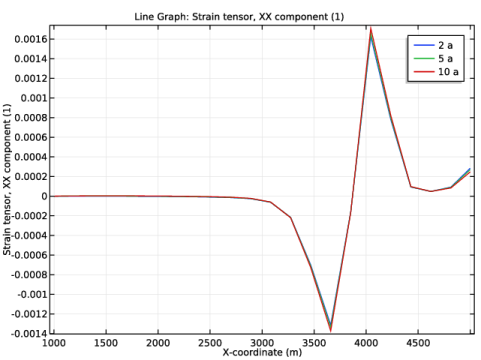
In the Settings window for Line Graph, click Replace Expression in the upper-right corner of the y-axis data section. From the menu, choose Model>Component 1>Solid Mechanics>Strain>Strain tensor (material and geometry frames)>solid.eXX - Strain tensor, XX component.
3
Locate the x-Axis Data section. From the Parameter list, choose Expression.
4
Click Replace Expression in the upper-right corner of the x-axis data section. From the menu, choose Model>Component 1>Geometry>Coordinate (material and geometry frames)>X - X-coordinate.
5
Click to expand the Legends section. Select the Show legends check box.
6
On the Horizontal Strain toolbar, click Plot.