|
|
|
|
Density ρ
|
|
|
|
|
|
|
|
|
|
|
1
|
|
2
|
|
3
|
Click Add.
|
|
4
|
Click Study.
|
|
5
|
|
6
|
Click Done.
|
|
1
|
|
2
|
|
1
|
|
2
|
|
3
|
|
4
|
|
5
|
|
6
|
|
7
|
|
1
|
|
2
|
Select the object cyl1 only.
|
|
3
|
|
4
|
|
5
|
|
1
|
|
2
|
|
1
|
|
2
|
|
3
|
|
5
|
|
6
|
|
1
|
|
2
|
|
3
|
|
1
|
Repeat above sequence of commands to add more Explicit selections using the information given in the following table:
|
|
2
|
|
1
|
In the Model Builder window’s toolbar, click the Show button and select Advanced Physics Options in the menu.
|
|
2
|
|
3
|
|
4
|
Select the Cavitation check box.
|
|
1
|
In the Model Builder window, under Component 1 (comp1)>Hydrodynamic Bearing (hdb) click Hydrodynamic Journal Bearing 1.
|
|
2
|
In the Settings window for Hydrodynamic Journal Bearing, type Hydrodynamic Journal Bearing (Plain) in the Label text field.
|
|
3
|
|
4
|
|
5
|
Locate the Fluid Properties section. From the μ list, choose User defined. In the associated text field, type mu.
|
|
1
|
Right-click Component 1 (comp1)>Hydrodynamic Bearing (hdb)>Hydrodynamic Journal Bearing (Plain) and choose Duplicate.
|
|
2
|
In the Settings window for Hydrodynamic Journal Bearing, type Hydrodynamic Journal Bearing (Elliptic) in the Label text field.
|
|
3
|
|
4
|
|
5
|
|
6
|
|
1
|
Right-click Component 1 (comp1)>Hydrodynamic Bearing (hdb)>Hydrodynamic Journal Bearing (Elliptic) and choose Duplicate.
|
|
2
|
In the Settings window for Hydrodynamic Journal Bearing, type Hydrodynamic Journal Bearing (Split halves) in the Label text field.
|
|
3
|
|
4
|
|
5
|
|
6
|
|
7
|
|
1
|
Right-click Component 1 (comp1)>Hydrodynamic Bearing (hdb)>Hydrodynamic Journal Bearing (Split halves) and choose Duplicate.
|
|
2
|
In the Settings window for Hydrodynamic Journal Bearing, type Hydrodynamic Journal Bearing (2-lobe) in the Label text field.
|
|
3
|
|
4
|
|
5
|
|
6
|
|
7
|
|
1
|
Right-click Component 1 (comp1)>Hydrodynamic Bearing (hdb)>Hydrodynamic Journal Bearing (2-lobe) and choose Duplicate.
|
|
2
|
In the Settings window for Hydrodynamic Journal Bearing, type Hydrodynamic Journal Bearing (3-lobe LOP) in the Label text field.
|
|
3
|
|
4
|
|
5
|
|
6
|
|
1
|
Right-click Component 1 (comp1)>Hydrodynamic Bearing (hdb)>Hydrodynamic Journal Bearing (3-lobe LOP) and choose Duplicate.
|
|
2
|
In the Settings window for Hydrodynamic Journal Bearing, type Hydrodynamic Journal Bearing (3-lobe LBP) in the Label text field.
|
|
3
|
|
1
|
Right-click Component 1 (comp1)>Hydrodynamic Bearing (hdb)>Hydrodynamic Journal Bearing (3-lobe LBP) and choose Duplicate.
|
|
2
|
In the Settings window for Hydrodynamic Journal Bearing, type Hydrodynamic Journal Bearing (4-lobe LOP) in the Label text field.
|
|
3
|
|
4
|
|
5
|
|
6
|
|
1
|
Right-click Component 1 (comp1)>Hydrodynamic Bearing (hdb)>Hydrodynamic Journal Bearing (4-lobe LOP) and choose Duplicate.
|
|
2
|
In the Settings window for Hydrodynamic Journal Bearing, type Hydrodynamic Journal Bearing (4-lobe LBP) in the Label text field.
|
|
3
|
|
1
|
|
2
|
In the Settings window for Bearing Orientation, type Bearing Orientation Hydrodynamic Journal Bearing (3-lobe LOP) in the Label text field.
|
|
3
|
|
4
|
|
1
|
|
2
|
In the Settings window for Bearing Orientation, type Bearing Orientation Hydrodynamic Journal Bearing (3-lobe LBP) in the Label text field.
|
|
3
|
|
4
|
|
1
|
Right-click Component 1 (comp1)>Hydrodynamic Bearing (hdb)>Bearing Orientation Hydrodynamic Journal Bearing (3-lobe LBP) and choose Duplicate.
|
|
2
|
In the Settings window for Bearing Orientation, type Bearing Orientation Hydrodynamic Journal Bearing (4-lobe LOP) in the Label text field.
|
|
3
|
|
4
|
|
1
|
|
2
|
|
3
|
|
4
|
|
5
|
|
1
|
In the Model Builder window, under Component 1 (comp1)>Hydrodynamic Bearing (hdb) click Hydrodynamic Journal Bearing (Plain).
|
|
2
|
|
3
|
|
1
|
In the Model Builder window, under Component 1 (comp1) right-click Mesh 1 and choose More Operations>Mapped.
|
|
2
|
|
3
|
|
1
|
|
2
|
|
3
|
|
4
|
|
5
|
|
6
|
|
1
|
|
2
|
|
3
|
Click Add.
|
|
5
|
|
1
|
|
2
|
|
3
|
|
4
|
|
1
|
|
2
|
|
3
|
|
4
|
|
1
|
|
2
|
|
3
|
|
4
|
|
5
|
|
6
|
|
7
|
|
8
|
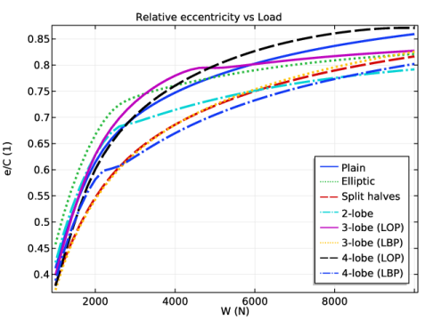
In the associated text field, type e/C (1).
|
|
1
|
|
2
|
|
4
|
Click to expand the Coloring and style section. Locate the Coloring and Style section. Find the Line style subsection. From the Line list, choose Cycle.
|
|
5
|
|
1
|
|
2
|
|
3
|
|
4
|
|
5
|
|
6
|
|
1
|
|
2
|
|
3
|
|
4
|
|
5
|
|
6
|
|
7
|
|
8
|
In the associated text field, type \phi (degree).
|
|
1
|
|
2
|
|
4
|
Click to expand the Coloring and style section. Locate the Coloring and Style section. Find the Line style subsection. From the Line list, choose Cycle.
|
|
5
|
|
1
|
|
2
|
|
3
|
|
4
|
|
1
|
|
2
|
|
3
|
|
4
|
|
5
|
|
6
|
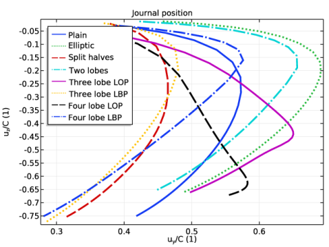
In the associated text field, type u<sub>y</sub>/C (1).
|
|
7
|
|
8
|
In the associated text field, type u<sub>z</sub>/C (1).
|
|
1
|
|
2
|
|
3
|
|
4
|
|
5
|
|
6
|
Click to expand the Coloring and style section. Locate the Coloring and Style section. Find the Line style subsection. From the Line list, choose Cycle.
|
|
7
|
|
8
|
|
1
|
|
2
|
|
3
|
|
4
|
|
5
|
Locate the Legends section. In the table, enter the following settings:
|
|
1
|
|
2
|
|
3
|
|
4
|
|
5
|
|
6
|
|
1
|
|
2
|
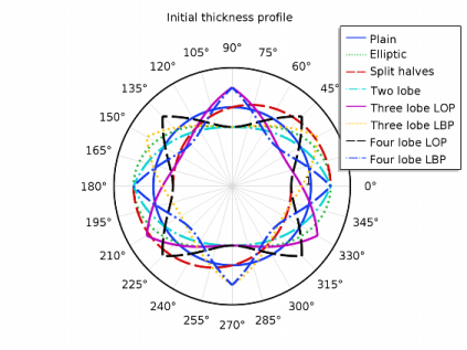
In the Settings window for Polar Plot Group, type Polar: Initial Thickness Profile in the Label text field.
|
|
3
|
|
4
|
|
5
|
|
6
|
|
7
|
|
8
|
|
1
|
|
3
|
|
4
|
|
5
|
Select the Description check box.
|
|
6
|
|
7
|
|
8
|
|
9
|
Click to expand the Coloring and style section. Locate the Coloring and Style section. Find the Line style subsection. From the Line list, choose Cycle.
|
|
10
|
|
11
|
|
12
|
|
14
|
|
1
|
|
2
|
|
3
|
|
5
|
|
6
|
Locate the Legends section. In the table, enter the following settings:
|
|
1
|
|
2
|
|
3
|
|
1
|
|
2
|
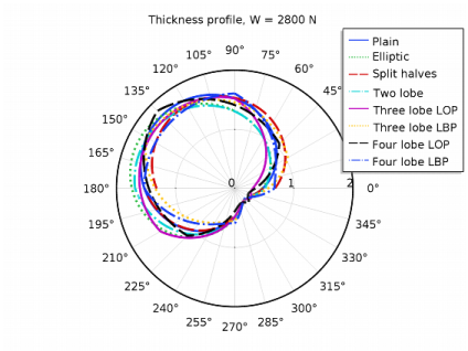
In the Settings window for Polar Plot Group, type Polar: Current Thickness Profile in the Label text field.
|
|
3
|
|
1
|
Edit the existing Line Graph nodes under Polar: Current Thickness Profile using the information given in the following table:
|
|
2
|
In the Model Builder window, expand the Results>Polar: Current Thickness Profile node, then click Polar: Current Thickness Profile.
|
|
3
|
|
4
|
|
5
|
|
6
|
|
7
|
|
8
|
|
9
|