|
|
|
|
1
|
|
2
|
|
3
|
Click Add.
|
|
4
|
Click Study.
|
|
5
|
|
6
|
Click Done.
|
|
1
|
|
2
|
|
1
|
|
2
|
|
1
|
|
2
|
|
3
|
|
4
|
|
6
|
|
7
|
|
8
|
|
1
|
|
2
|
|
3
|
|
4
|
|
6
|
Click Add.
|
|
8
|
|
1
|
|
2
|
|
3
|
|
4
|
|
1
|
|
2
|
|
3
|
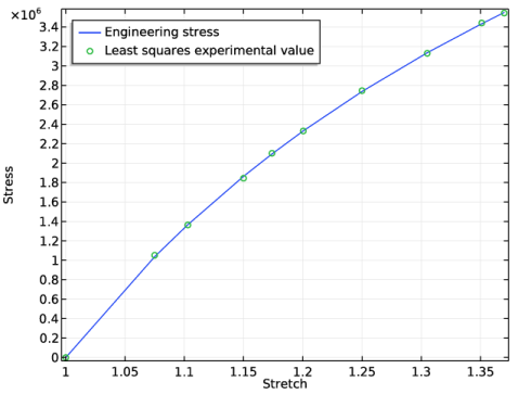
Click comp1.opt.glsobj1.col1 - Least squares experimental value in the upper-right corner of the section. Click to expand the Coloring and style section. Locate the Coloring and Style section. Find the Line style subsection. From the Line list, choose None.
|
|
4
|
|
5
|
|
6
|
|
1
|
|
2
|
|
3
|
|
4
|
|
5
|
In the associated text field, type Stretch.
|
|
6
|
|
7
|
|
8
|
|
1
|
|
2
|
|
3
|
|
4
|
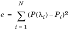
Click Replace Expression in the upper-right corner of the Expressions section. From the menu, choose Solver>Control parameters>C10 - Mooney-Rivlin parameter.
|
|
5
|
Click Evaluate.
|
|
6
|
Click Replace Expression in the upper-right corner of the Expressions section. From the menu, choose Solver>Control parameters>C01 - Mooney-Rivlin parameter.
|
|
7
|
Click Evaluate.
|