PDF

Benchmark Model of Molecular Flow Through an S-Bend
Introduction
Computing molecular flows in arbitrary geometries produces complex integral equations that are very difficult to compute analytically. There are two widely used methods for modeling molecular flows, the Monte Carlo method (which computes the trajectories of large numbers of randomized particles through the system) and the angular coefficient method. The Free Molecular Flow interfaces uses the angular coefficient method, which computes the molecular flow by summing the flux arriving at a surface from all other surfaces in its line of sight. The macroscopic variables in the vicinity of the surface can be derived from kinetic theory. The Particle Tracing Module can be used to implement the Monte Carlo method for molecular flows.
Note: This application requires the Particle Tracing Module.
Model Definition
This model compares the transmission probability, computed by two different methods of a gas through an s-bend geometry. The model geometry is shown in Figure 1.
Figure 1: Model geometry for the s-bend. The dimensions are in centimeters.
Particle trajectories are computed using Newton’s law of motion:
The particle velocity is given by:
When the particles encounter a boundary, they scatter according to Knudsen’s law.
where the subscript t denotes the tangential component of the velocity and n the normal. In addition, c is the particle speed and θ is the angle between the wall normal and the particle velocity. The particle speed is sampled from the following probability density function:
This is accomplished using the normally distributed random function, which is used to assign a new normally distributed random speed to each particle at each time step. The angle, θ is a random angle:
where Γ is a uniformly distributed random number between 0 and 1. Furthermore, it is unique for each particle at each time step. In all 10,000 particles are released into the modeling domain. The number of particles that reaches the outlet boundary determines the transmission probability.
The transmission probability for the molecular flow interface is given by the following:
(1)
One of the most important features of the Free Molecular Flow interface is its ability to reconstruct the number density on domains. This is done by evaluating an integral equation for each mesh element. Denoting the distance vector between the boundary and the centroid of each mesh element in the domain by r the number density can be defined as:
(2)
where the integration is carried out over all boundaries in the model. The expression changes slightly for the 3D case. The quantity is the rate of emission of molecules per unit area is the boundary normal, and is the inverse mean speed of the gas molecules. For more information, see the “Theory for the Free Molecular Flow Interface” in the Molecular Flow Module User’s Guide.
Results and Discussion
The incident molecular flux on the exterior boundaries is shown in Figure 2. Using Equation 2 the reconstructed number density is shown in Figure 3.
Figure 2: Plot of the incident molecular flux in the s-bend.
Figure 3: Plot of the reconstructed number density inside the s-bend.
The transmission probability for the molecular flow interface is 0.19676 and 0.1992 for the particle tracing. The two computed values are in close agreement. Note that slightly different results may be obtained for the particle tracing model each time the model is solved because random numbers are used so heavily in the computation.
When a Monte Carlo method is used to estimate the number density in the modeling domain, the results are in agreement with the reconstructed number density of Figure 3, as shown in Figure 4.
Figure 4: Comparison of the number density from the Molecular Flow and Particle Tracing Modules.
Notes About the COMSOL Implementation
The model is solved in two stages. First the Free Molecular Flow interface is used to compute the transmission probability using a Stationary study. Subsequently, the Mathematical Particle Tracing interface is used to compute the transmission probability with a Time Dependent study using a Monte Carlo approach. An Accumulator feature is applied to the domain to estimate the number density of particles.
Application Library path: Molecular_Flow_Module/Benchmarks/s_bend_benchmark
Modeling Instructions
From the File menu, choose New.
New
In the New window, click Model Wizard.
Model Wizard
1
In the Model Wizard window, click 2D.
2
In the Select Physics tree, select Fluid Flow>Rarefied Flow>Free Molecular Flow (fmf).
3
Click Add.
4
Click Study.
5
In the Select Study tree, select Preset Studies>Stationary.
6
Click Done.
Geometry 1
1
In the Model Builder window, under Component 1 (comp1) click Geometry 1.
2
In the Settings window for Geometry, locate the Units section.
3
From the Length unit list, choose cm.
Create the bends in the geometry by taking the difference of concentric circles
Rectangle 1 (r1)
1
On the Geometry toolbar, click Primitives and choose Rectangle.
2
In the Settings window for Rectangle, locate the Size and Shape section.
3
In the Width text field, type 2.
4
Right-click Rectangle 1 (r1) and choose Build Selected.
Circle 1 (c1)
1
On the Geometry toolbar, click Primitives and choose Circle.
2
In the Settings window for Circle, locate the Size and Shape section.
3
In the Sector angle text field, type 90.
4
Locate the Position section. In the x text field, type 2.
5
In the y text field, type 2.
6
Locate the Rotation Angle section. In the Rotation text field, type 270.
7
Right-click Circle 1 (c1) and choose Build Selected.
8
Click the Zoom Extents button on the Graphics toolbar.
Circle 2 (c2)
1
Right-click Circle 1 (c1) and choose Duplicate.
2
In the Settings window for Circle, locate the Size and Shape section.
3
In the Radius text field, type 2.
4
Right-click Component 1 (comp1)>Geometry 1>Circle 2 (c2) and choose Build Selected.
5
Click the Zoom Extents button on the Graphics toolbar.
Difference 1 (dif1)
1
On the Geometry toolbar, click Booleans and Partitions and choose Difference.
2
3
In the Settings window for Difference, locate the Difference section.
4
Find the Objects to subtract subsection. Select the Active toggle button.
5
6
Right-click Difference 1 (dif1) and choose Build Selected.
Circle 3 (c3)
1
On the Geometry toolbar, click Primitives and choose Circle.
2
In the Settings window for Circle, locate the Size and Shape section.
3
In the Sector angle text field, type 90.
4
Locate the Position section. In the x text field, type 5.
5
In the y text field, type 2.
6
Locate the Rotation Angle section. In the Rotation text field, type 90.
7
Right-click Circle 3 (c3) and choose Build Selected.
Circle 4 (c4)
1
Right-click Circle 3 (c3) and choose Duplicate.
2
In the Settings window for Circle, locate the Size and Shape section.
3
In the Radius text field, type 2.
4
Right-click Component 1 (comp1)>Geometry 1>Circle 4 (c4) and choose Build Selected.
5
Click the Zoom Extents button on the Graphics toolbar.
Difference 2 (dif2)
1
On the Geometry toolbar, click Booleans and Partitions and choose Difference.
2
3
In the Settings window for Difference, locate the Difference section.
4
Find the Objects to subtract subsection. Select the Active toggle button.
5
6
Click Build All Objects.
Rectangle 2 (r2)
1
On the Geometry toolbar, click Primitives and choose Rectangle.
2
In the Settings window for Rectangle, locate the Size and Shape section.
3
In the Width text field, type 2.
4
Locate the Position section. In the x text field, type 5.
5
In the y text field, type 3.
6
Click Build All Objects.
7
Click the Zoom Extents button on the Graphics toolbar.
Union 1 (uni1)
1
On the Geometry toolbar, click Booleans and Partitions and choose Union.
2
Click in the Graphics window and then press Ctrl+A to select all objects.
3
In the Settings window for Union, locate the Union section.
4
Clear the Keep interior boundaries check box.
5
Click Build All Objects.
The built geometry should appear as in Figure 1.
6
Click the Zoom Extents button on the Graphics toolbar.
Now add some parameters for the gas temperature and molecular weight.
Global Definitions
Parameters
1
On the Home toolbar, click Parameters.
2
In the Settings window for Parameters, locate the Parameters section.
3
Free Molecular Flow (fmf)
Molecular Flow 1
1
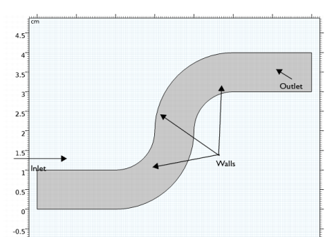
In the Model Builder window, under Component 1 (comp1)>Free Molecular Flow (fmf) click Molecular Flow 1.
2
In the Settings window for Molecular Flow, locate the Molecular Weight of Species section.
3
In the Mn, G text field, type Mw.
Surface Temperature 1
1
In the Model Builder window, under Component 1 (comp1)>Free Molecular Flow (fmf) click Surface Temperature 1.
2
In the Settings window for Surface Temperature, locate the Surface Temperature section.
3
In the T text field, type T0.
Reservoir 1
1
In the Model Builder window, right-click Free Molecular Flow (fmf) and choose Reservoir.
2
3
In the Settings window for Reservoir, locate the Reservoir section.
4
In the p0,G text field, type p_in.
Total Vacuum 1
1
Right-click Free Molecular Flow (fmf) and choose Total Vacuum.
2
The number density inside the domain can be reconstructed by adding the Number Density Reconstruction feature.
Number Density Reconstruction 1
1
Right-click Free Molecular Flow (fmf) and choose the domain setting Number Density Reconstruction.
2
Click in the Graphics window and then press Ctrl+A to select all domains.
In order to compute the transmission probability, only the molecular flux needs to be computed. To save some computation time, specify in the physics interface not to compute the pressure.
3
In the Model Builder window, click Free Molecular Flow (fmf).
4
In the Settings window for Free Molecular Flow, locate the Compute section.
5
Clear the Pressure check box.
6
Locate the Integration Settings section. From the Integration resolution list, choose 512.
Add integration component couplings on the inlet and outlet.
Definitions
Integration 1 (intop1)
1
On the Definitions toolbar, click Component Couplings and choose Integration.
2
In the Settings window for Integration, locate the Source Selection section.
3
From the Geometric entity level list, choose Boundary.
4
Integration 2 (intop2)
1
On the Definitions toolbar, click Component Couplings and choose Integration.
2
In the Settings window for Integration, locate the Source Selection section.
3
From the Geometric entity level list, choose Boundary.
4
Add expressions to compute the transmission probability using Equation 1
Variables 1
1
On the Definitions toolbar, click Local Variables.
2
In the Settings window for Variables, locate the Variables section.
3
Mesh 1
1
In the Model Builder window, under Component 1 (comp1) click Mesh 1.
2
In the Settings window for Mesh, locate the Mesh Settings section.
3
From the Element size list, choose Extremely fine.
4
Click Build All.
5
Click the Zoom Extents button on the Graphics toolbar.
Study 1
On the Home toolbar, click Compute.
Results
Incident Molecular Flux (fmf)
Click the Zoom Extents button on the Graphics toolbar.
2D Plot Group 3
1
On the Home toolbar, click Add Plot Group and choose 2D Plot Group.
2
In the Settings window for 2D Plot Group, type Number Density (fmf) in the Label text field.
Surface 1
1
Right-click Number Density (fmf) and choose Surface.
2
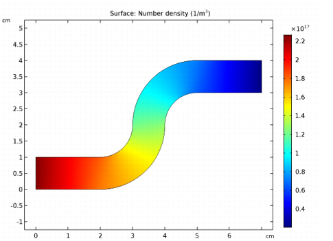
In the Settings window for Surface, click Replace Expression in the upper-right corner of the Expression section. From the menu, choose Model>Component 1>Free Molecular Flow>Number density>fmf.n_G - Number density.
3
On the Number Density (fmf) toolbar, click Plot.
4
Click the Zoom Extents button on the Graphics toolbar.
Now evaluate the transmission probability.
Global Evaluation 1
1
On the Results toolbar, click Global Evaluation.
2
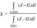
In the Settings window for Global Evaluation, click Replace Expression in the upper-right corner of the Expressions section. From the menu, choose Model>Component 1>Definitions>Variables>alpha - Transmission probability.
3
Click Evaluate.
Now add the Charged Particle Tracing interface to compute the transmission probability and number density using a Monte Carlo approach.
Add Physics
1
On the Home toolbar, click Add Physics to open the Add Physics window.
2
Go to the Add Physics window.
3
In the tree, select Mathematics>Mathematical Particle Tracing (pt).
It is possible to compute the transmission probability using the Mathematical Particle Tracing interface. However, the Charged Particle Tracing interface can also be used to estimate the number density within the domain.
4
Find the Physics interfaces in study subsection. In the table, clear the Solve check box for Study 1.
5
Click Add to Component in the window toolbar.
6
On the Home toolbar, click Add Physics to close the Add Physics window.
Add Study
1
On the Home toolbar, click Add Study to open the Add Study window.
2
Go to the Add Study window.
3
Find the Studies subsection. In the Select Study tree, select Preset Studies>Time Dependent.
4
Find the Physics interfaces in study subsection. In the table, clear the Solve check box for the Free Molecular Flow (fmf) interface.
5
Click Add Study in the window toolbar.
6
On the Home toolbar, click Add Study to close the Add Study window.
Mathematical Particle Tracing (pt)
On the Physics toolbar, click Free Molecular Flow (fmf) and choose Mathematical Particle Tracing (pt).
1
In the Model Builder window, under Component 1 (comp1) click Mathematical Particle Tracing (pt).
2
In the Settings window for Mathematical Particle Tracing, locate the Particle Release and Propagation section.
3
In the Maximum number of secondary particles text field, type 0.
Global Definitions
Parameters
1
In the Model Builder window, under Global Definitions click Parameters.
2
In the Settings window for Parameters, locate the Parameters section.
3
Definitions
Create a normally distributed random number with zero mean and standard deviation corresponding to the thermal velocity of the particles.
Random 1 (rn1)
1
On the Home toolbar, click Functions and choose Local>Random.
2
In the Settings window for Random, locate the Parameters section.
3
From the Distribution list, choose Normal.
4
In the Number of arguments text field, type 3.
5
In the Standard deviation text field, type cs.
Now define expressions for the particle velocity after it makes contact with the wall. The function random is a built in function to generate a uniformly distributed random number between -0.5 and 0.5 for an arbitrary number of input arguments. The variable pt.pidx is a built-in variable and is unique for each particle. The expression random(pt.pidx,t[1/s],1) will create a unique random number for each particle at each timestep.
Variables 2
1
On the Home toolbar, click Variables and choose Local Variables.
2
In the Settings window for Variables, locate the Variables section.
3
Mathematical Particle Tracing (pt)
Outlet 1
1
In the Model Builder window, under Component 1 (comp1) right-click Mathematical Particle Tracing (pt) and choose Outlet.
2
Inlet 1
1
In the Model Builder window, right-click Mathematical Particle Tracing (pt) and choose Inlet.
2
3
In the Settings window for Inlet, locate the Initial Position section.
4
From the Initial position list, choose Density.
5
In the N text field, type Np.
6
Locate the Initial Velocity section. Specify the v0 vector as
Wall 2
1
Right-click Mathematical Particle Tracing (pt) and choose Wall.
2
3
In the Settings window for Wall, locate the Wall Condition section.
4
From the Wall condition list, choose Disappear.
Wall 1
1
In the Model Builder window, under Component 1 (comp1)>Mathematical Particle Tracing (pt) click Wall 1.
2
In the Settings window for Wall, locate the Wall Condition section.
3
From the Wall condition list, choose General reflection.
4
Locate the General Reflection Settings section. Select the Specify tangential and normal velocity components check box.
5
Specify the vp vector as
Particle Counter 1
1
In the Model Builder window, right-click Mathematical Particle Tracing (pt) and choose the boundary condition Particle Counter.
2
3
In the Settings window for Particle Counter, locate the Particle Counter section.
4
From the Release feature list, choose Inlet 1.
Particle Properties 1
1
In the Model Builder window, under Component 1 (comp1)>Mathematical Particle Tracing (pt) click Particle Properties 1.
2
In the Settings window for Particle Properties, locate the Particle Mass section.
3
In the mp text field, type M.
Accumulator 1
1
In the Model Builder window, right-click Mathematical Particle Tracing (pt) and choose Accumulator.
2
Click in the Graphics window and then press Ctrl+A to select all domains.
3
In the Settings window for Accumulator, locate the Accumulator Settings section.
4
From the Accumulate over list, choose Elements and time.
5
In the Accumulated variable name text field, type Nd.
6
Locate the Units section. Find the Dependent variable quantity subsection. From the list, choose Number density (1/m^3).
7
Locate the Accumulator Settings section. In the R text field, type J_in*L/Np.
Study 2
Step 1: Time Dependent
1
In the Model Builder window, under Study 2 click Step 1: Time Dependent.
2
In the Settings window for Time Dependent, locate the Study Settings section.
3
Click Range.
4
In the Range dialog box, choose Number of values from the Entry method list.
5
In the Stop text field, type 0.006.
6
In the Number of values text field, type 30.
7
Click Replace.
8
On the Home toolbar, click Compute.
Results
Global Evaluation 2
1
On the Results toolbar, click Global Evaluation.
2
In the Settings window for Global Evaluation, locate the Data section.
3
From the Data set list, choose Study 2/Solution 2 (sol2).
4
From the Time selection list, choose Last.
5
Click Replace Expression in the upper-right corner of the Expressions section. From the menu, choose Model>Component 1>Mathematical Particle Tracing>Particle Counter 1>pt.pcnt1.alpha - Transmission probability.
6
Click Evaluate.
Table
1
Go to the Table window.
The transmission probability from the particle tracing approach agrees very well with the result from the Free Molecular Flow interface.
Results
Number Density (fmf)
1
In the Model Builder window, under Results right-click Number Density (fmf) and choose Duplicate.
 
Number Density (fmf) 1
1
In the Settings window for 2D Plot Group, type Number Density Comparison in the Label text field.
2
Click to expand the Title section. From the Title type list, choose None.
Number Density Comparison
In the Model Builder window, expand the Results>Number Density Comparison node.
Surface 2
1
Right-click Results>Number Density Comparison and choose Surface.
2
In the Settings window for Surface, locate the Data section.
3
From the Data set list, choose Particle 1.
4
Locate the Expression section. In the Expression text field, type pt.Nd.
5
Click to expand the Quality section. From the Resolution list, choose No refinement.
6
Click to expand the Inherit style section. Locate the Inherit Style section. From the Plot list, choose Surface 1.
Deformation 1
1
Right-click Results>Number Density Comparison>Surface 2 and choose Deformation.
2
In the Settings window for Deformation, locate the Expression section.
3
In the x component text field, type 0.
4
In the y component text field, type 4.
5
Locate the Scale section. Select the Scale factor check box.
6
Line 1
1
In the Model Builder window, under Results right-click Number Density Comparison and choose Line.
2
In the Settings window for Line, locate the Coloring and Style section.
3
From the Coloring list, choose Uniform.
4
From the Color list, choose Black.
Deformation 1
In the Model Builder window, under Results>Number Density Comparison>Surface 2 right-click Deformation 1 and choose Copy.
Surface 2
1
In the Model Builder window, under Results>Number Density Comparison right-click Line 1 and choose Paste Deformation.
2
In the Model Builder window, under Results>Number Density Comparison click Surface 2.
3
On the Number Density Comparison toolbar, click Plot.
4
Click the Zoom Extents button on the Graphics toolbar.
The results from the Mathematical Particle Tracing interface agree with the number density computed using the Free Molecular Flow interface.