PDF

Star-Shaped Microchannel
Introduction
Lab-on-a-chip devices have become quite popular for analyses in fields such as biochemistry and bioengineering. Through various techniques they incorporate all the equipment involved in a chemical process such as chemical reactors, heat exchangers, separators, and mixers.
This example involves the design of an infuser, a device that feeds a reactor or analysis equipment with a specific amount of fluid. Controlling pressure is an accurate way to introduce a set quantity of fluid at a certain velocity to some piece of equipment.
Flushing the equipment can also be important. Optimizing such an infuser to maximize its use would involve spending the least amount of time (and fluid) flushing the equipment. Modeling this process in the time domain can lead to an optimization of the infusing pressure, microchannel design, and time control.
This model demonstrates two useful tools in COMSOL Multiphysics modeling:
Model Definition
This exercise arbitrarily sets the geometry and conditions of the microchannel lab-on-a-chip (Figure 1). The differential pressure at the five inlets relative to the outlet pressure is time-controlled so that the inlet flow passes from one to the next in a smooth way. At any particular instant, one of the inlet flows dominates, although flow could be significant from more than one inlet. The pressure at the outlet is set to zero.
Figure 1: Model geometry for a star-shaped infuser with five inlets and one outlet. The model sets up a varying pressure differential at each inlet in the time domain in such a way that the dominant inlet flow alternates among them.
The example models only fluid flow whose velocity is of a magnitude that suggests laminar behavior. This implies that you can get a numerical solution of the full momentum balance and continuity equations for incompressible flow with a reasonable number of elements. The equations you must solve are the Navier-Stokes equations in the time domain
where ρ denotes density (kg/m3), u is the velocity (m/s), μ denotes dynamic viscosity (Pa·s), and p equals pressure (Pa). The fluid in this case is water, with the corresponding density and viscosity values.
The boundary conditions for the inlets and the outlet assume a set pressure; they also assume vanishing viscous stress:
Set the pressure at the outlet to zero; at the inlets, use the time-dependent expressions
where  t is time (s), and k is a value between zero and one. This simplified example sets the phase α to 0, π/4, π/2, 3π/4, or π, depending on the inlet boundary.
Apply the no slip condition to all other boundaries; it states that the velocity is zero in the x, y, and z directions at the wall:
Results
Figure 2 shows the velocity field as a combined slice and arrow plot through the middle of the geometry at t = 0.5 s. Setting up and observing this plot as an animation gives an informative qualitative description of the process.
Figure 2: The velocity field in a microchannel infuser through the middle of the geometry.
Figure 3 shows the velocity in the x direction and the pressure in a point near the outlet as functions of time.
Figure 3: Velocity in the x direction (top) and pressure (bottom) at a point near the outlet.
Notes About the COMSOL Implementation
This example illustrates how to use time-dependent boundary conditions to simulate a changing process. You can implement this scenario using a boundary condition that is a function of time. The physics interface provides direct access to the built-in time variable (t) and the mathematical functions you need.
In 3D models, results at the walls are important but they can also hide what occurs within the geometry. This example also illustrates how to better display results with the help of hidden boundaries.
Finally, this model approaches meshing in a way that deviates from the default settings. In most cases COMSOL Multiphysics automatically generates a 3D mesh made completely of tetrahedrons. Here—as is the case in many other microchannels and minichannels—the top and the bottom boundaries are significant in modeling the flow profile because the distance between them is of the same magnitude as that between the two sides. This means that you must model the device in 3D. However, because the microchannel’s height does not change along its length, the software does not require much meshing to resolve this dimension.
As an alternative to its default meshing, it is possible to extrude a mesh. To illustrate this concept, you create the mesh in this model by first taking a cross section of the full geometry to construct a 2D geometry. After meshing that, you then extrude the geometry and sweep the mesh in the height dimension. This approach provides some mesh and memory conservation.
Application Library path: Microfluidics_Module/Fluid_Flow/star_chip
Modeling Instructions
From the File menu, choose New.
New
In the New window, click Model Wizard.
Model Wizard
1
In the Model Wizard window, click 3D.
2
In the Select Physics tree, select Fluid Flow>Single-Phase Flow>Laminar Flow (spf).
3
Click Add.
4
Click Study.
5
In the Select Study tree, select Preset Studies>Stationary.
6
Click Done.
Geometry 1
1
In the Model Builder window, under Component 1 (comp1) click Geometry 1.
2
In the Settings window for Geometry, locate the Units section.
3
From the Length unit list, choose µm.
Work Plane 1 (wp1)
1
On the Geometry toolbar, click Work Plane.
2
In the Settings window for Work Plane, click Show Work Plane.
Bézier Polygon 1 (b1)
1
On the Work Plane toolbar, click Primitives and choose Bézier Polygon.
2
In the Settings window for Bézier Polygon, locate the General section.
3
From the Type list, choose Open curve.
4
Locate the Polygon Segments section. Find the Added segments subsection. Click Add Linear.
5
Find the Control points subsection. In row 1, set xw to 325 and yw to 12.5.
6
In row 2, set xw to 325 and yw to 25.
7
Find the Added segments subsection. Click Add Linear.
8
Find the Control points subsection. In row 2, set xw to 30.
9
Find the Added segments subsection. Click Add Linear.
10
Find the Control points subsection. In row 2, set xw to 0 and yw to 30.
11
Find the Added segments subsection. Click Add Linear.
12
Find the Control points subsection. In row 2, set yw to 150.
13
Find the Added segments subsection. Click Add Linear.
14
Find the Control points subsection. In row 2, set xw to -25.
15
Find the Added segments subsection. Click Add Linear.
16
Find the Control points subsection. In row 2, set yw to 55.
17
Find the Added segments subsection. Click Add Linear.
18
Find the Control points subsection. In row 2, set xw to -97 and yw to 125.
19
Find the Added segments subsection. Click Add Linear.
20
Find the Control points subsection. In row 2, set xw to -115 and yw to 110.
21
Find the Added segments subsection. Click Add Linear.
22
Find the Control points subsection. In row 2, set xw to -30 and yw to 25.
23
Find the Added segments subsection. Click Add Linear.
24
Find the Control points subsection. In row 2, set xw to -150.
25
Find the Added segments subsection. Click Add Linear.
26
Find the Control points subsection. In row 2, set yw to 12.5.
27
Find the Added segments subsection. Click Add Linear.
28
Find the Control points subsection. In row 2, set xw to -30.
29
Find the Added segments subsection. Click Add Linear.
30
Locate the General section. From the Type list, choose Solid.
31
Right-click Bézier Polygon 1 (b1) and choose Build Selected.
Mirror 1 (mir1)
1
On the Work Plane toolbar, click Transforms and choose Mirror.
2
3
In the Settings window for Mirror, locate the Input section.
4
Select the Keep input objects check box.
5
Locate the Point on Line of Reflection section. In the xw text field, type 82.5.
6
In the yw text field, type 12.5.
7
Locate the Normal Vector to Line of Reflection section. In the xw text field, type 0.
8
In the yw text field, type 1.
9
Right-click Mirror 1 (mir1) and choose Build Selected.
Union 1 (uni1)
1
On the Work Plane toolbar, click Booleans and Partitions and choose Union.
2
Click in the Graphics window and then press Ctrl+A to select both objects.
3
In the Settings window for Union, locate the Union section.
4
Clear the Keep interior boundaries check box.
5
Right-click Union 1 (uni1) and choose Build Selected.
Work Plane 1 (wp1)
In the Model Builder window, under Component 1 (comp1)>Geometry 1 click Work Plane 1 (wp1).
Extrude 1 (ext1)
1
On the Geometry toolbar, click Extrude.
2
In the Settings window for Extrude, locate the Distances section.
3
4
Click Build All Objects.
5
Click the Zoom Extents button on the Graphics toolbar.
Mesh 1
Extruding a 2D mesh into 3D creates a more structured mesh than the default.
Size
1
In the Model Builder window, under Component 1 (comp1) right-click Mesh 1 and choose Swept.
2
In the Settings window for Size, locate the Element Size section.
3
From the Calibrate for list, choose Fluid dynamics.
Distribution 1
1
In the Model Builder window, under Component 1 (comp1)>Mesh 1 right-click Swept 1 and choose Distribution.
2
In the Settings window for Distribution, locate the Distribution section.
3
In the Number of elements text field, type 8.
4
Click in the Graphics window and then press Ctrl+A to select all domains.
5
Click Build All.
Global Definitions
Parameters
1
On the Home toolbar, click Parameters.
2
In the Settings window for Parameters, locate the Parameters section.
3
Definitions
Variables 1
1
On the Home toolbar, click Variables and choose Local Variables.
2
In the Settings window for Variables, locate the Variables section.
3
Materials
Material 1 (mat1)
1
In the Model Builder window, under Component 1 (comp1) right-click Materials and choose Blank Material.
2
In the Settings window for Material, locate the Material Contents section.
3
Laminar Flow (spf)
Inlet 1
1
In the Model Builder window, under Component 1 (comp1) right-click Laminar Flow (spf) and choose Inlet.
2
3
In the Settings window for Inlet, locate the Boundary Condition section.
4
5
Locate the Pressure Conditions section. In the p0 text field, type p_in_c.
Inlet 2
1
In the Model Builder window, right-click Laminar Flow (spf) and choose Inlet.
2
3
In the Settings window for Inlet, locate the Boundary Condition section.
4
5
Locate the Pressure Conditions section. In the p0 text field, type p_in_ir.
Inlet 3
1
Right-click Laminar Flow (spf) and choose Inlet.
2
3
In the Settings window for Inlet, locate the Boundary Condition section.
4
5
Locate the Pressure Conditions section. In the p0 text field, type p_in_il.
Inlet 4
1
Right-click Laminar Flow (spf) and choose Inlet.
2
3
In the Settings window for Inlet, locate the Boundary Condition section.
4
5
Locate the Pressure Conditions section. In the p0 text field, type p_in_rm.
Inlet 5
1
Right-click Laminar Flow (spf) and choose Inlet.
2
3
In the Settings window for Inlet, locate the Boundary Condition section.
4
5
Locate the Pressure Conditions section. In the p0 text field, type p_in_lm.
Outlet 1
1
Right-click Laminar Flow (spf) and choose Outlet.
2
Study 1
Step 2: Time Dependent
1
On the Study toolbar, click Study Steps and choose Time Dependent>Time Dependent.
2
In the Settings window for Time Dependent, locate the Study Settings section.
3
In the Times text field, type range(0,0.1,4).
4
On the Study toolbar, click Compute.
Results
Velocity (spf)
Next, reproduce the plot in Figure 2, showing the velocity field at t = 0.5 s as a combined slice and arrow plot.
1
In the Model Builder window, under Results click Velocity (spf).
2
In the Settings window for 3D Plot Group, locate the Data section.
3
From the Time (s) list, choose 0.5.
4
Locate the Plot Settings section. Clear the Plot data set edges check box.
This setting gives an unobstructed view of the slice you will specify, which shows the shape of the microchannel chip.
Slice
1
In the Model Builder window, expand the Velocity (spf) node, then click Slice.
2
In the Settings window for Slice, locate the Expression section.
3
From the Unit list, choose mm/s.
4
Locate the Plane Data section. From the Plane list, choose XY-planes.
5
In the Planes text field, type 1.
6
On the Velocity (spf) toolbar, click Plot.
Arrow Volume 1
1
In the Model Builder window, under Results right-click Velocity (spf) and choose Arrow Volume.
2
In the Settings window for Arrow Volume, locate the Arrow Positioning section.
3
Find the X grid points subsection. In the Points text field, type 35.
4
Find the Y grid points subsection. In the Points text field, type 35.
5
Find the Z grid points subsection. In the Points text field, type 1.
6
Locate the Coloring and Style section. From the Arrow length list, choose Normalized.
7
Select the Scale factor check box.
8
9
On the Velocity (spf) toolbar, click Plot.
Pressure (spf)
The second default plot shows the surface of the geometry with the pressure as a contour plot.
1
In the Model Builder window, under Results click Pressure (spf).
2
In the Settings window for 3D Plot Group, locate the Data section.
3
From the Time (s) list, choose 0.5.
4
On the Pressure (spf) toolbar, click Plot.
5
Click the Zoom Extents button on the Graphics toolbar.
Data Sets
To create the plots in Figure 3 showing the velocity in the x direction and the pressure at a point near the outlet, perform the following steps:
Cut Point 3D 1
1
On the Results toolbar, click Cut Point 3D.
2
In the Settings window for Cut Point 3D, locate the Point Data section.
3
In the X text field, type 275.
4
In the Y text field, type 12.5.
5
In the Z text field, type 12.5.
1D Plot Group 3
1
On the Results toolbar, click 1D Plot Group.
2
In the Settings window for 1D Plot Group, locate the Data section.
3
From the Data set list, choose Cut Point 3D 1.
Point Graph 1
1
Right-click 1D Plot Group 3 and choose Point Graph.
2
In the Settings window for Point Graph, locate the Data section.
3
From the Data set list, choose Cut Point 3D 1.
4
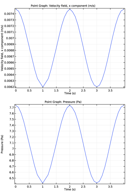
Click Replace Expression in the upper-right corner of the y-axis data section. From the menu, choose Model>Component 1>Laminar Flow>Velocity and pressure>Velocity field>u - Velocity field, x component.
5
On the 1D Plot Group 3 toolbar, click Plot.
Point Graph 1
1
In the Model Builder window, under Results right-click 1D Plot Group 3 and choose Duplicate.
2
In the Model Builder window, expand the 1D Plot Group 4 node, then click Point Graph 1.
3
In the Settings window for Point Graph, click Replace Expression in the upper-right corner of the y-axis data section. From the menu, choose Model>Component 1>Laminar Flow>Velocity and pressure>p - Pressure.
4
On the 1D Plot Group 4 toolbar, click Plot.