|
|
|

|
1
|
|
2
|
In the Select Physics tree, select Heat Transfer>Radiation>Heat Transfer with Surface-to-Surface Radiation (ht).
|
|
3
|
Click Add.
|
|
4
|
Click Study.
|
|
5
|
|
6
|
Click Done.
|
|
1
|
|
2
|
|
1
|
|
2
|
|
3
|
|
1
|
|
2
|
|
3
|
|
4
|
Click to expand the Layers section. In the table, enter the following settings:
|
|
5
|
|
1
|
|
2
|
On the object c1, select Boundaries 1–12 only.
|
|
3
|
|
1
|
|
2
|
|
3
|
|
4
|
|
5
|
|
6
|
|
7
|
|
1
|
|
2
|
|
3
|
|
4
|
|
5
|
|
6
|
|
7
|
|
1
|
|
2
|
|
3
|
|
4
|
|
5
|
|
1
|
|
2
|
On the object uni1, select Points 1, 4, 5, and 8–10 only.
|
|
3
|
|
4
|
|
5
|
|
1
|
|
2
|
|
3
|
|
4
|
|
5
|
|
6
|
Click to expand the Layers section. In the table, enter the following settings:
|
|
7
|
|
1
|
|
2
|
|
3
|
|
4
|
On the object c2, select Domain 1 only.
|
|
1
|
|
2
|
|
3
|
|
4
|
Click Range.
|
|
5
|
|
6
|
|
7
|
|
8
|
Click Replace.
|
|
9
|
|
1
|
|
2
|
|
1
|
|
2
|
|
3
|
|
4
|
|
5
|
Click OK.
|
|
1
|
|
2
|
|
3
|
|
1
|
|
2
|
|
4
|
|
1
|
|
2
|
|
3
|
|
4
|
|
1
|
|
2
|
|
4
|
|
1
|
|
2
|
|
3
|
In the tree, select Built-In>Air.
|
|
4
|
|
1
|
|
3
|
|
1
|
|
3
|
|
4
|
|
1
|
|
2
|
|
3
|
|
4
|
|
5
|
Locate the Surface Emissivity section. From the ε list, choose User defined. In the associated text field, type 0.01.
|
|
1
|
|
3
|
|
4
|
|
5
|
|
1
|
|
3
|
|
4
|
|
5
|
Locate the Surface Emissivity section. From the ε list, choose User defined. In the associated text field, type 0.1.
|
|
1
|
|
3
|
|
4
|
|
5
|
Locate the Surface Emissivity section. From the ε list, choose User defined. In the associated text field, type 0.1.
|
|
1
|
|
3
|
|
4
|
|
1
|
|
3
|
|
4
|
|
5
|
Locate the Surface Emissivity section. From the ε list, choose User defined. In the associated text field, type 0.99.
|
|
1
|
|
3
|
|
4
|
|
1
|
|
3
|
|
4
|
|
5
|
Locate the Surface Emissivity section. From the ε list, choose User defined. In the associated text field, type 0.99.
|
|
1
|
|
3
|
|
4
|
|
1
|
|
2
|
|
1
|
|
2
|
|
3
|
|
4
|
|
1
|
In the Model Builder window, under Component 1 (comp1)>Mesh 1 right-click Free Triangular 1 and choose Size.
|
|
2
|
|
3
|
|
4
|
|
5
|
|
6
|
|
7
|
|
8
|
|
9
|
|
10
|
|
1
|
|
2
|
|
3
|
|
1
|
In the Model Builder window, under Component 1 (comp1)>Mesh 1 right-click Free Triangular 1 and choose Size.
|
|
2
|
|
3
|
|
5
|
|
6
|
|
7
|
|
8
|
|
9
|
|
10
|
|
1
|
|
2
|
|
3
|
Click Add.
|
|
4
|
Click Range.
|
|
5
|
|
6
|
|
7
|
|
8
|
Click Replace.
|
|
9
|
|
1
|
|
2
|
|
3
|
In the Model Builder window, expand the Study 1>Solver Configurations>Solution 1 (sol1)>Stationary Solver 1 node, then click Parametric 1.
|
|
4
|
|
5
|
|
6
|
|
1
|
|
1
|
|
2
|
|
3
|
|
1
|
|
3
|
|
1
|
|
2
|
|
3
|
|
1
|
|
3
|
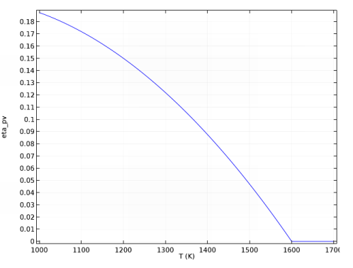
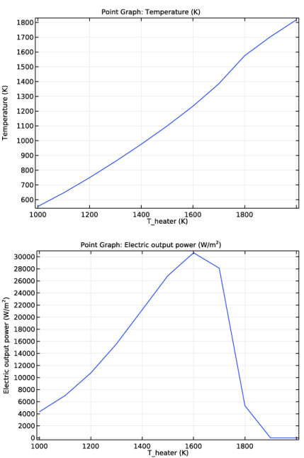
In the Settings window for Point Graph, click Replace Expression in the upper-right corner of the y-axis data section. From the menu, choose Model>Component 1>Definitions>Variables>q_out - Electric output power.
|
|
4
|
|
1
|
|
2
|
|
3
|
|
4
|
|
1
|
|
2
|
|
3
|
|
4
|
|
5
|
|
1
|
|
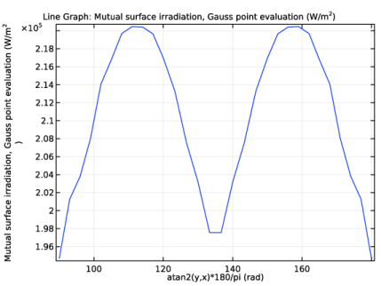
3
|
In the Settings window for Line Graph, click Replace Expression in the upper-right corner of the y-axis data section. From the menu, choose Model>Component 1>Heat Transfer with Surface-to-Surface Radiation>Radiation>Mutual surface irradiation>ht.Gm_gp - Mutual surface irradiation, Gauss point evaluation.
|
|
4
|
|
5
|
|
6
|
|
7
|
|
8
|