|
|
|
|
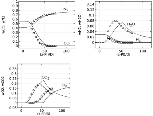
N2
|
||||
|
H2
|
||||
|
O2
|
||||
|
CO2
|
|
1
|
|
2
|
In the Select Physics tree, select Fluid Flow>Single-Phase Flow>Turbulent Flow>Turbulent Flow, k-ω (spf).
|
|
3
|
Click Add.
|
|
4
|
Click Study.
|
|
5
|
|
6
|
Click Done.
|
|
1
|
|
2
|
|
3
|
|
4
|
Browse to the model’s Application Libraries folder and double-click the file round_jet_burner_params.txt.
|
|
1
|
|
2
|
|
3
|
|
4
|
|
5
|
|
6
|
|
1
|
|
2
|
|
3
|
|
4
|
|
1
|
In the Model Builder window, under Component 1 (comp1)>Turbulent Flow, k-ω (spf) click Fluid Properties 1.
|
|
2
|
|
3
|
|
4
|
|
1
|
|
3
|
|
4
|
|
5
|
|
1
|
|
3
|
|
4
|
|
1
|
|
2
|
|
4
|
|
5
|
|
6
|
|
7
|
|
8
|
|
1
|
|
3
|
|
4
|
|
5
|
|
6
|
|
7
|
|
8
|
|
1
|
|
2
|
|
3
|
|
4
|
Find the Physics interfaces in study subsection. In the table, clear the Solve check box for Study 1.
|
|
5
|
Click to expand the Dependent variables section. Locate the Dependent Variables section. In the Number of species text field, type 6.
|
|
6
|
In the Mass fractions table, enter the following settings:
|
|
7
|
|
8
|
|
9
|
|
10
|
Find the Physics interfaces in study subsection. In the table, clear the Solve check box for Study 1.
|
|
11
|
|
12
|
|
1
|
|
2
|
|
3
|
Find the Select the physics interfaces you want to couple subsection. In the table, enter the following settings:
|
|
4
|
|
5
|
|
6
|
|
7
|
|
1
|
In the Model Builder window, under Component 2 (comp2)>Multiphysics click Nonisothermal Flow 1 (nitf1).
|
|
2
|
|
3
|
|
4
|
|
5
|
|
1
|
|
2
|
|
3
|
|
4
|
|
5
|
|
1
|
|
2
|
|
3
|
|
4
|
Browse to the model’s Application Libraries folder and double-click the file round_jet_burner_vars.txt.
|
|
1
|
|
2
|
|
3
|
|
4
|
|
5
|
|
1
|
|
2
|
|
3
|
|
4
|
|
5
|
|
6
|
|
1
|
|
2
|
On the object r2, select Points 3 and 4 only.
|
|
3
|
|
4
|
|
5
|
|
6
|
|
1
|
|
2
|
|
3
|
|
4
|
|
5
|
|
6
|
|
7
|
|
8
|
|
9
|
|
1
|
|
2
|
|
3
|
|
4
|
|
5
|
|
1
|
|
2
|
Select the object uni1 only.
|
|
3
|
|
4
|
|
5
|
Select the object cha1 only.
|
|
6
|
|
1
|
|
2
|
|
3
|
|
4
|
|
5
|
|
6
|
|
1
|
|
2
|
|
3
|
|
4
|
|
5
|
|
6
|
|
1
|
|
2
|
On the object fin, select Boundaries 6 and 11 only.
|
|
3
|
|
4
|
|
1
|
|
2
|
On the object mce1, select Boundaries 3 and 11 only.
|
|
3
|
|
1
|
|
2
|
Click in the Graphics window and then press Ctrl+A to select all domains.
|
|
3
|
|
4
|
Select the Active toggle button.
|
|
6
|
Select the Active toggle button.
|
|
8
|
|
9
|
|
11
|
Select the Active toggle button.
|
|
1
|
In the Model Builder window, under Component 2 (comp2)>Turbulent Flow, k-ω 2 (spf2) click Fluid Properties 1.
|
|
2
|
|
3
|
|
1
|
|
3
|
|
4
|
|
5
|
|
6
|
|
7
|
|
1
|
|
3
|
|
4
|
|
5
|
|
6
|
|
7
|
|
1
|
|
3
|
|
4
|
|
1
|
In the Model Builder window, under Component 2 (comp2) click Transport of Concentrated Species (tcs).
|
|
2
|
In the Settings window for Transport of Concentrated Species, locate the Transport Mechanisms section.
|
|
3
|
|
4
|
|
1
|
In the Model Builder window, under Component 2 (comp2)>Transport of Concentrated Species (tcs) click Transport Properties 1.
|
|
2
|
|
3
|
|
4
|
|
5
|
|
6
|
|
7
|
|
8
|
|
9
|
|
1
|
In the Model Builder window, under Component 2 (comp2)>Transport of Concentrated Species (tcs) click Initial Values 1.
|
|
2
|
|
3
|
|
4
|
|
5
|
|
6
|
|
7
|
|
1
|
|
3
|
|
4
|
|
5
|
|
6
|
|
7
|
|
8
|
|
9
|
|
1
|
|
3
|
|
4
|
|
5
|
|
6
|
|
7
|
|
8
|
|
1
|
|
1
|
|
2
|
Click in the Graphics window and then press Ctrl+A to select all domains.
|
|
3
|
|
4
|
|
5
|
|
6
|
|
7
|
|
8
|
|
9
|
|
1
|
|
2
|
|
3
|
|
4
|
|
5
|
|
6
|
|
1
|
|
2
|
|
3
|
|
5
|
Locate the Interpolation and Extrapolation section. From the Interpolation list, choose Piecewise cubic.
|
|
6
|
|
7
|
|
8
|
Click Plot.
|
|
1
|
|
2
|
|
3
|
|
1
|
|
2
|
|
3
|
|
1
|
|
2
|
|
3
|
|
1
|
|
2
|
|
3
|
|
1
|
|
2
|
|
3
|
|
1
|
|
2
|
|
1
|
|
2
|
|
3
|
From the k list, choose User defined. In the associated text field, type k_mix+Cp_mix*spf2.muT/0.72.
|
|
4
|
|
5
|
|
6
|
|
1
|
In the Model Builder window, under Component 2 (comp2)>Heat Transfer in Fluids (ht) click Initial Values 1.
|
|
2
|
|
3
|
|
1
|
|
3
|
|
4
|
|
1
|
|
1
|
|
2
|
Click in the Graphics window and then press Ctrl+A to select all domains.
|
|
3
|
|
4
|
|
1
|
|
2
|
In the Model Builder window, under Component 2 (comp2) right-click Mesh 2 and choose Edit Physics-Induced Sequence.
|
|
1
|
|
2
|
|
3
|
Click the Custom button.
|
|
4
|
|
5
|
|
6
|
|
1
|
|
2
|
|
3
|
Click the Custom button.
|
|
4
|
|
6
|
|
1
|
|
2
|
|
3
|
Click the Custom button.
|
|
4
|
Locate the Geometric Entity Selection section. From the Geometric entity level list, choose Boundary.
|
|
6
|
|
8
|
|
1
|
|
2
|
|
3
|
|
1
|
In the Model Builder window, expand the Boundary Layers 1 node, then click Boundary Layer Properties 1.
|
|
2
|
|
3
|
|
4
|
|
1
|
|
2
|
|
1
|
In the Model Builder window, expand the Solution 1 (sol1) node, then click Study 2>Step 1: Stationary.
|
|
2
|
|
3
|
In the table, clear the Solve for check box for Turbulent Flow, k-ω (spf) and Heat Transfer in Fluids (ht).
|
|
4
|
Click to expand the Values of dependent variables section. Locate the Values of Dependent Variables section. Find the Values of variables not solved for subsection. From the Settings list, choose User controlled.
|
|
5
|
|
6
|
|
1
|
|
2
|
|
3
|
In the Model Builder window, expand the Study 2>Solver Configurations>Solution 2 (sol2)>Stationary Solver 1 node.
|
|
4
|
In the Model Builder window, under Study 2>Solver Configurations>Solution 2 (sol2)>Stationary Solver 1 click Segregated 1.
|
|
5
|
|
6
|
|
7
|
|
8
|
|
9
|
In the Model Builder window, under Study 2>Solver Configurations>Solution 2 (sol2)>Stationary Solver 1>Segregated 1 click Velocity u2, Pressure p2.
|
|
10
|
|
11
|
|
12
|
In the Add dialog box, In the Variables list, choose Wall temperature (comp2.nitf1.TWall_d), Wall temperature (comp2.nitf1.TWall_u), and Temperature (comp2.T).
|
|
13
|
Click OK.
|
|
14
|
In the Model Builder window, under Study 2>Solver Configurations>Solution 2 (sol2)>Stationary Solver 1>Segregated 1 click Segregated Step 2.
|
|
15
|
|
16
|
|
17
|
|
18
|
In the Model Builder window, under Study 2>Solver Configurations>Solution 2 (sol2)>Stationary Solver 1>Segregated 1 right-click Segregated Step 3 and choose Disable.
|
|
1
|
|
2
|
|
3
|
|
1
|
|
2
|
|
3
|
|
1
|
|
2
|
|
3
|
|
1
|
|
2
|
|
3
|
|
1
|
|
2
|
|
3
|
|
4
|
|
5
|
|
6
|
Click to expand the Advanced section. Find the Space variable subsection. In the x text field, type r_mirr20.
|
|
1
|
|
2
|
|
3
|
|
4
|
Locate the Advanced section. Find the Space variable subsection. In the x text field, type r_mirr50.
|
|
1
|
|
2
|
|
3
|
|
4
|
|
5
|
|
1
|
|
2
|
|
3
|
|
4
|
|
5
|
|
6
|
|
7
|
|
1
|
|
2
|
|
3
|
|
4
|
|
1
|
|
2
|
|
3
|
|
4
|
|
1
|
|
2
|
|
3
|
|
4
|
|
5
|
|
1
|
|
2
|
|
3
|
|
4
|
|
5
|
|
1
|
|
2
|
|
3
|
|
1
|
|
2
|
|
3
|
|
4
|
|
1
|
|
2
|
|
3
|
Click Import.
|
|
4
|
Browse to the model’s Application Libraries folder and double-click the file round_jet_burner_chnAclY.fav.
|
|
1
|
Go to the Table window.
|
|
2
|
|
3
|
|
4
|
Click OK.
|
|
1
|
|
2
|
|
3
|
Click Import.
|
|
4
|
Browse to the model’s Application Libraries folder and double-click the file round_jet_burner_chnAd20Y.fav.
|
|
1
|
Go to the Table window.
|
|
2
|
|
3
|
|
4
|
Click OK.
|
|
1
|
|
2
|
|
3
|
Click Import.
|
|
4
|
Browse to the model’s Application Libraries folder and double-click the file round_jet_burner_chnAd50Y.fav.
|
|
1
|
Go to the Table window.
|
|
2
|
|
3
|
|
4
|
Click OK.
|
|
1
|
|
2
|
|
3
|
Click Import.
|
|
4
|
Browse to the model’s Application Libraries folder and double-click the file round_jet_burner_seq1420.dat.
|
|
1
|
Go to the Table window.
|
|
2
|
|
3
|
|
4
|
Click OK.
|
|
1
|
|
2
|
|
3
|
Click Import.
|
|
4
|
Browse to the model’s Application Libraries folder and double-click the file round_jet_burner_seq1450.dat.
|
|
1
|
Go to the Table window.
|
|
2
|
|
3
|
|
4
|
Click OK.
|
|
1
|
|
2
|
|
3
|
|
1
|
|
3
|
|
4
|
|
5
|
|
6
|
|
7
|
Click to expand the Coloring and style section. Locate the Coloring and Style section. From the Color list, choose Black.
|
|
8
|
|
9
|
|
1
|
|
2
|
|
3
|
|
4
|
|
5
|
|
6
|
Click to expand the Preprocessing section. Find the x-axis column subsection. From the Preprocessing list, choose Linear.
|
|
7
|
|
8
|
|
9
|
|
10
|
Locate the Coloring and Style section. Find the Line style subsection. From the Line list, choose None.
|
|
11
|
|
12
|
|
13
|
|
14
|
|
15
|
|
1
|
|
2
|
|
3
|
Click OK.
|
|
4
|
|
5
|
|
6
|
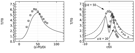
In the associated text field, type (z-Pl)/Di.
|
|
7
|
|
9
|
|
10
|
|
11
|
|
12
|
|
13
|
|
14
|
|
15
|
|
16
|
|
1
|
|
2
|
|
3
|
|
1
|
|
2
|
|
3
|
|
4
|
|
5
|
|
6
|
|
7
|
Click to expand the Coloring and style section. Locate the Coloring and Style section. From the Color list, choose Black.
|
|
8
|
|
9
|
|
1
|
|
2
|
|
3
|
|
4
|
|
5
|
Locate the Coloring and Style section. Find the Line style subsection. From the Line list, choose Dashed.
|
|
6
|
Locate the Legends section. In the table, enter the following settings:
|
|
7
|
|
1
|
|
2
|
|
3
|
|
4
|
|
5
|
|
6
|
|
7
|
Click to expand the Preprocessing section. Find the x-axis column subsection. From the Preprocessing list, choose Linear.
|
|
8
|
|
9
|
|
10
|
|
11
|
Click to expand the Coloring and style section. Locate the Coloring and Style section. Find the Line style subsection. From the Line list, choose None.
|
|
12
|
|
13
|
|
14
|
|
15
|
|
16
|
|
1
|
|
2
|
|
3
|
|
4
|
Locate the Coloring and Style section. Find the Line markers subsection. From the Marker list, choose Triangle.
|
|
5
|
Locate the Legends section. In the table, enter the following settings:
|
|
1
|
|
2
|
|
3
|
Click OK.
|
|
4
|
|
5
|
|
6
|
|
7
|
|
9
|
|
10
|
|
11
|
|
12
|
|
13
|
|
14
|
|
15
|
|
16
|
|
1
|
|
2
|
|
3
|
|
4
|
Click OK.
|
|
1
|
|
2
|
|
3
|
|
1
|
|
2
|
|
3
|
|
1
|
|
2
|
|
3
|
|
4
|
|
5
|
|
6
|
Locate the Preprocessing section. Find the y-axis columns subsection. From the Preprocessing list, choose Linear.
|
|
7
|
|
1
|
|
2
|
|
3
|
|
4
|
|
5
|
|
6
|
Locate the Preprocessing section. Find the y-axis columns subsection. From the Preprocessing list, choose Linear.
|
|
7
|
|
1
|
|
2
|
|
3
|
|
4
|
|
5
|
|
6
|
|
7
|
|
8
|
|
9
|
|
10
|
|
1
|
|
2
|
|
3
|
|
4
|
Click OK.
|
|
5
|
|
6
|
|
7
|
|
8
|
|
9
|
|
10
|
|
11
|
|
1
|
|
2
|
|
3
|
|
4
|
Locate the Legends section. In the table, enter the following settings:
|
|
1
|
|
2
|
|
3
|
|
4
|
Locate the Preprocessing section. Find the y-axis columns subsection. In the Scaling text field, type 1.
|
|
5
|
Locate the Legends section. In the table, enter the following settings:
|
|
6
|
|
1
|
In the Model Builder window, under Results>CO, N2 @ centerline right-click Line Graph 1 and choose Duplicate.
|
|
2
|
|
3
|
|
4
|
Click to expand the Coloring and style section. Locate the Coloring and Style section. Find the Line style subsection. From the Line list, choose Dashed.
|
|
5
|
Locate the Legends section. In the table, enter the following settings:
|
|
1
|
In the Model Builder window, under Results>CO, N2 @ centerline right-click Table Graph 1 and choose Duplicate.
|
|
2
|
|
3
|
|
4
|
Locate the Coloring and Style section. Find the Line markers subsection. From the Marker list, choose Triangle.
|
|
5
|
Locate the Legends section. In the table, enter the following settings:
|
|
6
|
|
1
|
|
2
|
|
3
|
|
4
|
Click OK.
|
|
1
|
|
2
|
|
3
|
|
4
|
Locate the Legends section. In the table, enter the following settings:
|
|
1
|
|
2
|
|
3
|
|
4
|
Locate the Legends section. In the table, enter the following settings:
|
|
1
|
|
2
|
|
3
|
|
4
|
Locate the Legends section. In the table, enter the following settings:
|
|
1
|
|
2
|
|
3
|
|
4
|
Locate the Legends section. In the table, enter the following settings:
|
|
1
|
|
2
|
|
3
|
|
4
|
|
5
|
|
6
|
|
7
|
|
1
|
|
2
|
|
3
|
|
4
|
Click OK.
|
|
1
|
|
2
|
|
3
|
|
4
|
Locate the Legends section. In the table, enter the following settings:
|
|
1
|
|
2
|
|
3
|
|
4
|
Locate the Legends section. In the table, enter the following settings:
|
|
1
|
|
2
|
|
3
|
|
4
|
Locate the Legends section. In the table, enter the following settings:
|
|
1
|
|
2
|
|
3
|
|
4
|
Locate the Legends section. In the table, enter the following settings:
|
|
1
|
|
2
|
|
3
|
|
4
|
|
5
|
|
6
|
|
7
|
Click Plot.
|