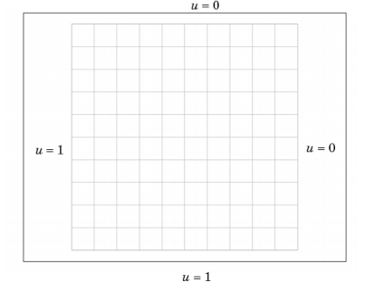
solved on the unit square. Equation 3-5 is discretized using
10 times
10 quadratic Lagrangian elements. The boundary conditions are:
Figure 3-23 shows the mesh and boundary conditions. In general, using uniform meshes for transport problems is not recommended. Nevertheless, this example uses a uniform mesh to demonstrate the different stabilization techniques.
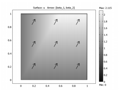
The expected solution rises slowly and smoothly from the left and lower boundaries and has sharp boundary layers along the upper and right boundaries. Figure 3-24 shows a reference solution obtained using
100-by-
100 quadratic Lagrangian elements with streamline diffusion and crosswind diffusion (see the next section). The arrows indicate the direction of
β.
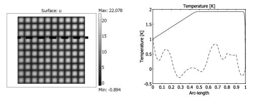
Figure 3-25 displays the solution obtained using the mesh in
Figure 3-23 and (unstabilized) Galerkin discretization. As can be expected with such a high Péclet number, the unstabilized solution shows little, if any, resemblance to the reference solution in
Figure 3-24. The right plot in
Figure 3-25 shows a cross-sectional plot along the dashed line,
y = 0.8 and the corresponding reference solution. Notice that the unstabilized solution is destroyed by oscillations.
The Stabilization Techniques section explores how different stabilization techniques affect the solution of this example.